第六次周报

week 6 内容：

• louis philippe morency 《多模态机器学习》 35%

• 论文阅读：

  1. DeepCoclustering
  2. AutoRec: Autoencoders Meet Collaborative Filtering
  3. AugGAN：Cross Domain Adaptation with GAN based DataAugmentation

DeepCoclustering（SDM 2019）

主要内容

framework

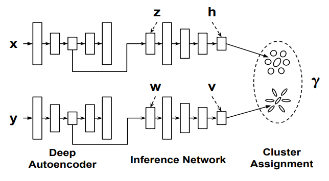
这篇文章提出了一种深度学习框架下的共聚类（co-clustering）方法，在聚类精度上超过了其他传统方法。

其中X代表instance（行，对应user)， Y代表features(列，对应item)， 分别进入Autoencoders进行降维（先进行pretrain 1000 epoch，然后利用encoder接入后面network进行端到端训练），将结果输入inference network（一个multi-layer neural network), 利用GMM框架进行cluster assignment。

优化目标

cluster assignment

参数和概率表示：

inference network：\(\eta_{r}\)、\(\eta_{c}\) ——》 \(Q_{\eta_{r}}(k|h_i)\) \(Q_{\eta_{c}}(k|v_j)\) (cluster assignment distributions)

GMM：\(\phi_{r}\)、\(\phi_{c}\) ——》\(P_{\phi_{r}}(k|h_i)\) \(P_{\phi_{c}}(k|v_j)\) (cluster assignment posterior)

对于AE输出的隐变量\(z_i\), 进入inference network中的MLN，得到\(h_i\):

​ \(\mathbf{h}_{i}=\operatorname{Softmax}\left(M L N\left(\mathbf{z}_{i} ; \eta_{r}\right)\right)\)

而后GMM第k个参数：\(\phi_{r}=\left\{\pi_{r}^{k}, \mu_{r}^{k}, \Sigma_{r}^{k}\right\}\),可以被表示为：

​ \(\begin{array}{l} \pi_{r}^{k}=N_{r}^{k} / N_{r}, \quad \mu_{r}^{k}=\frac{1}{N_{r}^{k}} \sum_{i=1}^{N_{r}^{k}} h_{i k} \mathbf{h}_{i} \\ \Sigma_{r}^{k}=\frac{1}{N_{r}^{k}} \sum_{i=1}^{N_{r}} h_{i k}\left(\mathbf{h}_{i}-\mu_{r}^{k}\right)\left(\mathbf{h}_{i}-\mu_{r}^{k}\right)^{T} \end{array}\)

其中\(N_{r}\)是instance的数目（即user），\(N_{r}^{k}\)是所有instance对应 \(h_i\)的 k-dim的和，这样第i个instance分配给第k个cluster的概率可以表示为：

​ \(\gamma_{r(i)}^{k}=\frac{\pi_{r}^{k} \mathcal{N}\left(\mathbf{h}_{i} \mid \mu_{r}^{k}, \Sigma_{r}^{k}\right)}{\sum_{k^{\prime}=1}^{g} \pi_{r}^{k^{\prime}} \mathcal{N}\left(\mathbf{h}_{i} \mid \mu_{r}^{k^{\prime}}, \Sigma_{r}^{k^{\prime}}\right)}\)

似然函数（取\(\gamma_{r(i)}^{k}\)上边求和）：

​ \(\log \left\{\prod_{i=1}^{N_{r}} P_{\phi_{r}}\left(\mathbf{h}_{i}\right)\right\}=\sum_{i=1}^{N_{r}} \log P_{\phi_{r}}\left(\mathbf{h}_{i}\right)=\sum_{i=1}^{N_{r}} \log \left\{\sum_{k=1}^{K} \pi_{r}^{k} \mathcal{N}\left(\mathbf{h}_{i} \mid \mu_{r}^{k}, \Sigma_{r}^{k}\right)\right\}\)

DeepCC并没有直接进行MLE，而是最大化变分lower bound，有两点优势：

1. 通过最小化Q P之间的KL散度，让GMM更准确

2. 与对数似然绑定，让训练过程更加effective

   lower bound:

​ \(\begin{array}{l} \sum_{i=1}^{N_{r}} \log P\left(\mathbf{h}_{i}\right)=\sum_{i=1}^{N_{r}} \log \int_{k} P\left(k, \mathbf{h}_{i}\right) \\ =\sum_{i=1}^{N_{r}} \log \int_{k} \frac{P\left(k, \mathbf{h}_{i}\right)}{Q\left(k \mid \mathbf{h}_{i}\right)} Q\left(k \mid \mathbf{h}_{i}\right) \\ =\sum_{i=1}^{N_{r}} \log \left(E_{Q}\left[\frac{P\left(k, \mathbf{h}_{i}\right)}{Q\left(k \mid \mathbf{h}_{i}\right)}\right]\right) \\ \geq \sum_{i=1}^{N_{r}} E_{Q}\left[\log \frac{P\left(k, \mathbf{h}_{i}\right)}{Q\left(k \mid \mathbf{h}_{i}\right)}\right] \\ =\sum_{i=1}^{N_{r}}\left\{E_{Q}\left[\log P\left(k, \mathbf{h}_{i}\right)\right]+H\left(k \mid \mathbf{h}_{i}\right)\right\} \\ =\mathcal{L}_{r} \end{array}\)

中间把log拿入期望使用了jensen ‘s inequality

更进一步，可以得到Q与P之间KL散度与lower bound关系(第二步减了一个\(logP(h_i)\)，又加了一个)：

\(\begin{array}{l} \mathcal{L}_{r}=\sum_{i=1}^{N_{r}}\left\{E_{Q}\left[\log P\left(k, \mathbf{h}_{i}\right)\right]-E_{Q}\left(\log Q\left(k \mid \mathbf{h}_{i}\right)\right)\right\} \\ =\sum_{i=1}^{N_{r}}\left\{\int_{k} Q\left(k \mid \mathbf{h}_{i}\right) \log \frac{P\left(k, \mathbf{h}_{i}\right)}{Q\left(k \mid \mathbf{h}_{i}\right)}-\right. \left.\int_{k} Q\left(k \mid \mathbf{h}_{i}\right) \log P\left(\mathbf{h}_{i}\right)+\log P\left(\mathbf{h}_{i}\right)\right\} \\ =\sum_{i=1}^{N_{r}}\left\{\int_{k} Q\left(k \mid \mathbf{h}_{i}\right) \log \frac{P\left(k, \mathbf{h}_{i}\right)}{Q\left(k \mid \mathbf{h}_{i}\right) P\left(\mathbf{h}_{i}\right)}+\log P\left(\mathbf{h}_{i}\right)\right\} \\ =\sum_{i=1}^{N_{r}}\left\{\int_{k} Q\left(k \mid \mathbf{h}_{i}\right) \log \frac{P\left(k \mid \mathbf{h}_{i}\right)}{Q\left(k \mid \mathbf{h}_{i}\right)}+\log P\left(\mathbf{h}_{i}\right)\right\} \\ =\sum_{i=1}^{N_{r}}\left\{-K L\left(Q\left(k \mid \mathbf{h}_{i}\right) \| P\left(k \mid \mathbf{h}_{i}\right)\right)+\log P\left(\mathbf{h}_{i}\right)\right\} \end{array}\)

对应可以得到feature的assignment loss：

\(\mathcal{L}_{c}=\sum_{j=1}^{N_{c}}\left\{E_{Q}\left[\log P\left(k, \mathbf{v}_{j}\right)\right]-E_{Q}\left(\log Q\left(k \mid \mathbf{v}_{j}\right)\right)\right\}\)

Instance-Feature Cross Loss

对联合概率\(P(X,Y)\)设计loss进行优化

assignment到cluster的概率：

instance: \(\gamma_{r(i)}=\left(\gamma_{r(i)}^{1}, \cdots, \gamma_{r(i)}^{g}\right)^{T}\)

feature：\(\gamma_{c(i)}=\left(\gamma_{c(i)}^{1}, \cdots, \gamma_{c(i)}^{g}\right)^{T}\)

第i个instance和第j个instance的联合概率（划分前）表示为：

\(p\left(\mathbf{x}_{i}, \mathbf{y}_{j}\right)=\mathcal{J}\left(\boldsymbol{\gamma}_{r(i)}, \boldsymbol{\gamma}_{c(j)}\right)\)

第s个instance cluster和第t个feature cluster的联合概率（划分后）为：

\(p\left(\hat{\mathbf{x}}_{s}, \hat{\mathbf{y}}_{t}\right)=\sum\left\{p\left(\mathbf{x}_{i}, \mathbf{y}_{j}\right) \mid \mathbf{x}_{i} \in \hat{\mathbf{x}}_{s}, \mathbf{y}_{j} \in \hat{\mathbf{y}}_{t}\right\}\)

在论文中，作者使用点积来表示\(\mathcal{J}\),其实是可以尝试改变的。这样做的原因有两点：

1. 大部分co-cluster， instance cluster以及feature cluster 数量是相等的
2. 相近的instance 有着相似的 feature

各自的互信息：

\(I(X ; Y)=\sum_{\mathbf{x}_{i}} \sum_{\mathbf{y}_{j}} p\left(\mathbf{x}_{i}, \mathbf{y}_{j}\right) \log \frac{p\left(\mathbf{x}_{i}, \mathbf{y}_{j}\right)}{p\left(\mathbf{x}_{i}\right) p\left(\mathbf{y}_{j}\right)}\)

\(I(\hat{X} ; \hat{Y})=\sum_{\hat{\mathbf{x}}_{s}} \sum_{\hat{\mathbf{y}}_{t}} p\left(\hat{\mathbf{x}}_{s}, \hat{\mathbf{y}}_{t}\right) \log \frac{p\left(\hat{\mathbf{x}}_{s}, \hat{\mathbf{y}}_{t}\right)}{p\left(\hat{\mathbf{x}}_{s}\right), p\left(\hat{\mathbf{y}}_{t}\right)}\)

互信息之间的差：\(I(X ; Y)-I(\hat{X} ; \hat{Y})\)

\(\begin{array}{l} =\sum_{\hat{\mathbf{x}}_{s}} \sum_{\hat{\mathbf{y}}_{t}} \sum_{\mathbf{x}_{i} \in \hat{\mathbf{x}}_{s}} \sum_{\mathbf{y}_{j} \in \hat{\mathbf{y}}_{t}} p\left(\mathbf{x}_{i}, \mathbf{x}_{j}\right) \log \frac{p\left(\mathbf{x}_{i}, \mathbf{x}_{j}\right)}{p\left(\mathbf{x}_{i}\right) p\left(\mathbf{x}_{j}\right)} \\ -\sum_{\hat{\mathbf{x}}_{s}} \sum_{\hat{\mathbf{y}}_{t}}\left(\sum_{\mathbf{x}_{i} \in \hat{\mathbf{x}}_{s}} \sum_{\mathbf{y}_{j} \in \hat{\mathbf{y}}_{t}} p\left(\mathbf{x}_{i}, \mathbf{y}_{j}\right)\right) \log \frac{p\left(\hat{\mathbf{x}}_{s}, \hat{\mathbf{y}}_{t}\right)}{p\left(\hat{\mathbf{x}}_{s}\right) p\left(\hat{\mathbf{y}}_{t}\right)} \\ =\sum_{\hat{\mathbf{x}}_{s}} \sum_{\hat{\mathbf{y}}_{t}} \sum_{\mathbf{x}_{i} \in \hat{\mathbf{x}}_{s}} \sum_{\mathbf{y}_{j} \in \hat{\mathbf{y}}_{t}} p\left(\mathbf{x}_{i}, \mathbf{y}_{j}\right) \log \frac{p\left(\mathbf{x}_{i}, \mathbf{y}_{j}\right)}{q\left(\mathbf{x}_{i}, \mathbf{y}_{j}\right)} \\ =K L(p(X, Y) \| q(X, Y)) \\ \geq 0 \end{array}\)

因此为了让差最小化（划分后损失最少），设计loss为：

​ \(1-\frac{I(\hat{X} ; \hat{Y})}{I(X ; Y)}\)

整体loss

综合上述loss：

\(\begin{array}{c} \quad \min _{\theta_{r}, \theta_{c}, \eta_{r}, \eta_{c}} J=J_{1}+J_{2}+J_{3} \\ J_{1}=\frac{\lambda_{1}}{n} \sum_{i=1}^{n} l\left(\mathbf{x}_{i}, g_{r}\left(\mathbf{z}_{i}\right)\right)+\lambda_{2} P_{a e}\left(\theta_{r}\right)+\lambda_{3}\left(-\mathcal{L}_{r}\right)+P_{i n f}\left(\Sigma_{r}\right) \\ J_{2}=\frac{\lambda_{1}}{d} \sum_{j=1}^{i} l\left(\mathbf{y}_{j}, g_{c}\left(\mathbf{w}_{j}\right)\right)+\lambda_{2} P_{a e}\left(\theta_{c}\right)+\lambda_{3}\left(-\mathcal{L}_{c}\right)+P_{\text {inf }}\left(\Sigma_{c}\right) \\ J_{3}=\lambda_{4}\left(1-\frac{I(\hat{X} ; \hat{Y})}{I(X ; X)}\right) \end{array}\)

AutoRec: Autoencoders Meet Collaborative Filtering（WWW 2015）

1、写作动机

2015年前后，深度神经网络在视觉（vision）和对话（speech）数据建模方面取得了显著的突破，该文作者由此产生了把深度神经网络应用到协同过滤模型的想法。该文基于自编码器提出了协同过滤模型AutoRec，并通过实验证明了该模型较此前的基于神经网络的协同过滤模型具有更强的表示能力和更高的计算效率。

2、问题定义

给定用户集合 、物品集合 、部分用户-物品评分记录构成的用户-物品评价矩阵，对未知用户-物品评价行为做评分预测，根据均方根误差（RMSE)做评估。

其模型也可以写成重建函数形式：

(1)

其中 和 分别为输出层和隐藏层的激活函数，参数集 , , , , . 对应 个用户和 个条目, 维隐藏层。

跟AutoEncoder类似地，其损失函数为

[公式]

不过考虑到对模型参数的限制，比如加入L2正则，损失函数变化为：

[公式]

其中 为Frobenius范数.

3、具体模型

img

如上图所示，该文提出的AutoRec模型采取了最简单的自编码器结构，通过一层神经网络编码输入特征得到隐藏层表示，再通过一层神经网络表示对隐藏层表示做解码还原输入特征。根据输入特征的不同，该模型可分为 和 ：输入特征为用户-物品评价矩阵的行，则为基于物品特征学习的自编码器 ；输入特征为用户-物品评价矩阵的列，则为基于用户特征学习的自编码器 。

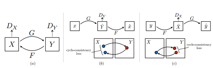
CycleGAN（ ICCV 2017）

pix2pix使用了pair的data进行训练，然而现实中往往是unpaired-data，CycleGAN就是希望能够在目标域和源域之间，不用建立一对一的映射，就可以完成迁移的训练。

img

做到这一点：

1. 需要有两个判别器， 分别判断X到Y与Y到X的生成，以及Y到X的生成。

2. cycle-consistency loss ，生成器可能会直接生成一张目标域的图像而无视源域图像，因此需要保证能够映射回X

   

   img

AugGAN：基于GAN的图像数据增强（ECCV 2018）

主要内容

augGan利用语义分割的结构意识（structure-aware）进行数据域的迁移。与cycleGan等进行风格迁移的image2image translation不同，这篇文章利用结构意识强调生成照片的真实性而非艺术性。

AugGAN的训练数据包含：1. 分割mask；2，不同领域的图像(春天和冬天，白天和黑夜)。

img

主要结构：

img

AugGan结构如上图：

1. 整体迁移是有方向的，X代表源域图像，Y代表目标域图像。$ E_x, E_y\(分别代表X和Y的encoder，将图像降维后会得到特征域Z，Z会对接两个decoder，分别输出预测的分割图\){},{}\(，以及生成的fake image\) {X},{Y}$。
2. augGan使用了cycleGan类似的循环结构，保证循环一致性，\(\bar{Y}\)经过\(E_y，G_y\)得到重构后的$ X_{rec}\(，对\){X}$同理。
3. 有两个判别器\(D_x,D_y\)
4. augGan对于decoder中的残差结构使用了hard-share权重共享，对于上采样的结构使用soft-share

loss 设计

总体loss:

\(\begin{aligned} \mathcal{L}_{\text {full }} &=\mathcal{L}_{G A N}\left(E_{x}, G_{x}, D_{x}, X, Y\right)+\mathcal{L}_{G A N}\left(E_{y}, G_{y}, D_{y}, Y, X\right) \\ &+\lambda_{\text {cyc }} * \mathcal{L}_{\text {cyc }}\left(E_{x}, G_{x}, E_{y}, G_{y}, X, Y\right) \\ &+\lambda_{\text {seg }} *\left(\mathcal{L}_{\text {seg }}\left(E_{x}, P_{x}, X, \hat{X}\right)+\mathcal{L}_{\text {seg }}\left(E_{y}, P_{y}, Y, \hat{Y}\right)\right) \\ &+\lambda_{\omega} *\left(\mathcal{L}_{\omega_{x}}\left(\omega_{G_{x}}, \omega_{P_{x}}\right)+\mathcal{L}_{\omega_{y}}\left(\omega_{G_{y}}, \omega_{P_{y}}\right)\right) \end{aligned}\)

1. 结构意识（structure-aware）

   在转换图像的时候，让模型明白不同位置是什么样的背景(语义特征)有利于迁移，AugGan使用分割的标签来实现。

   \(\begin{aligned} \mathcal{L}_{\text {seg }-x}\left(P_{x}, E_{x}, X, \hat{X}\right) &=\lambda_{\text {seg-L1 }} \mathbb{E}_{x \sim p_{\text {data }(x)}}\left[\left\|P_{x}\left(E_{x}(x)\right)-\hat{x}\right\|_{1}\right] \\ &+\lambda_{\text {seg-crossentropy }} \mathbb{E}_{x \sim p_{\text {data }(x)}}\left[\left\|\log \left(P_{x}\left(E_{x}(x)\right)-\hat{x}\right)\right\|_{1}\right] \end{aligned}\)

   L1loss以及交叉熵损失

2. 权值共享

   hard-sharing: 完全共享一样的权值

   soft-sharing：通过loss进行约束

   $ {}({G}, {P})=-(({G_{x}} {P{x}} /|{G{x}}|{2}|{P_{x}}|_{2})^{2}) $

3. 循环一致性(Cycle consistency)

   生成的图片经过重新编码解码能够还原回原来的图片，这样可以保证P(z|X)不会退化为P(z)（不会随机生成目标域的图像）。

   \(\begin{aligned} \mathcal{L}_{c y c}\left(E_{x}, G_{x}, E_{y}, G_{y}, X, Y\right) &=\mathbb{E}_{x \sim p_{\text {data }(x)}}\left[\left\|G_{y}\left(E_{y}\left(G_{x}\left(E_{x}(x)\right)\right)\right)-\mathrm{x}\right\|_{1}\right] \\ &+\mathbb{E}_{y \sim p_{\text {data }(y)}}\left[\left\|G_{x}\left(E_{x}\left(G_{y}\left(E_{y}(y)\right)\right)\right)-y\right\|_{1}\right] \end{aligned}\)

4. 对抗训练

​ 论文中对抗训练使用了原始的GanLoss：

​ \(\begin{aligned} \mathcal{L}_{G A N_{1}}\left(E_{x}, G_{x}, D_{x}, X, Y\right) &=\mathbb{E}_{y \sim p_{\text {data }(y)}}\left[\log D_{x}(y)\right] \\ &+\mathbb{E}_{x \sim p_{\text {data }(x)}}\left[\log \left(1-D_{x}\left(G_{x}\left(E_{x}(x)\right)\right)\right)\right] \end{aligned}\)

迁移效果

img